How does Stable Diffusion AI work?

Stable Diffusion is a deep learning model. Stable Diffusion is a text-to-image model in its most basic version. It will provide an image that matches the text if you give it a text prompt.
We shall delve deeply into the inner workings of stable diffusion. What is the purpose of knowing? You will become a better artist if you have some knowledge of the inner workings of things, which is intriguing in and of itself. If you utilise the tool appropriately, you can get results with greater accuracy.
Stable Diffusion and Diffusion Models
Stable Diffusion is a member of the Diffusion model class of deep learning models. Additionally, they are generative models, which means they are made to produce new data that resembles the training data. Images serve as the data in the case of stable diffusion.
Its name, diffusion model, explains why. This is because the math closely resembles the physics of diffusion.
Let’s imagine that we solely used the images of cats and dogs to train our diffusion model. The groupings of cat and dog photos are shown in the figure below as the two peaks on the left.
Forward Diffusion in Stable Diffusion AI
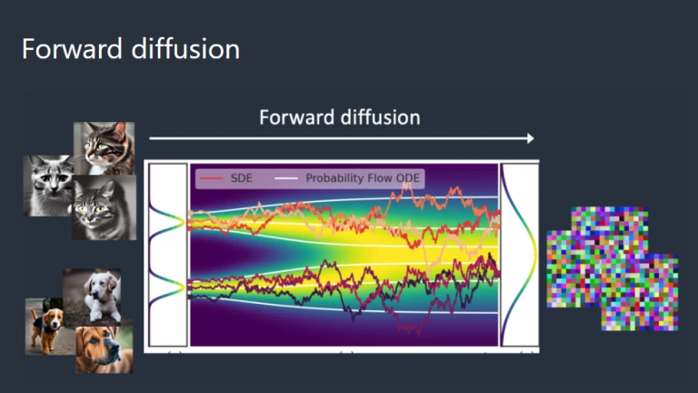 Forward Diffusion
A training image gradually becomes an atypical noise image after being subjected to a forward diffusion technique that introduces noise. Any image of a cat or dog will become a noisy image thanks to the forward process. You won’t be able to determine whether they were a dog or a cat at first in the end. (This is crucial.)
This is comparable to an ink drop landing in a glass of water. In water, the ink drop diffuses. After some time, It disperses itself haphazardly throughout the lake. It is no longer possible to determine whether it dropped at the centre or close to the rim initially.
Thus, the image that is experiencing forward diffusion is seen below. The cat image becomes erratic noise.
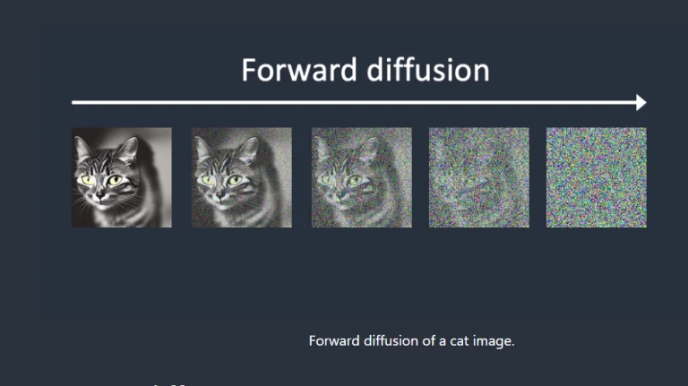 Forward Diffusion- Cat
Reverse Diffusion in Stable Diffusion AI
The intriguing portion is about to start. What if the diffusion could be reversed? Similar to reverse-playing a video. Time-traveling in the past. We’ll check to see where the ink drop was first put in.
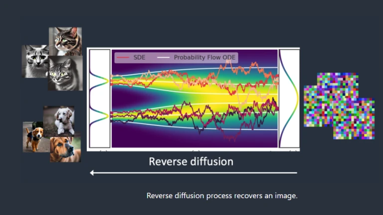 Reverse Diffusion
Reverse diffusion recovers a cat OR a dog picture from a noisy, meaningless image. This is the central notion.
Thus, each diffusion process technically consists of two stages: (1) drift or directed motion, and (2) random motion. In the opposite dispersion, there are no images other than cats or dogs. Because of this, the outcome might be either a dog or a cat.
Training for Reverse Diffusion
Reverse diffusion is an intelligent and beautiful concept. But how can it be done is a million-dollar question.
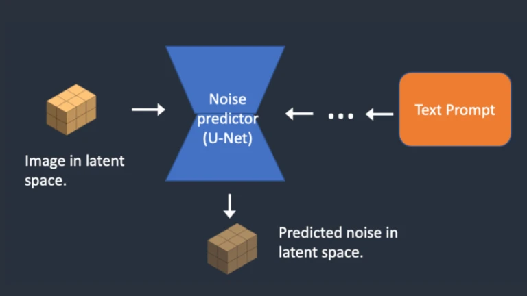
We need to know how much noise is introduced to an image in order to reverse diffusion. The solution is to train a neural network model to forecast the additional noise. In stable diffusion, it is referred to as the noise predictor. The model is a U-Net. The training proceeds as follows:
- Choose a training image, such as a picture of a cat.
- Make a picture of random noise.
- Add this noisy image to the training image up to a predetermined number of times to distort it.
- Teach the noise predictor to inform us of the overall noise the altered image has added. By adjusting its weights and displaying the right response, this is accomplished.
- We now have a noise predictor that can calculate the amount of noise introduced to an image after training.
Before asking the noise predictor to identify the noise, we first create a totally random image. The original image is then adjusted to account for this estimated noise. Continue doing this several times. You will either see a cat or a dog in the result.
Stable Diffusion AI Model
We must now break some bad news to you: What we just discussed is NOT how Stable Diffusion AI operates! The aforementioned diffusion process is in picture space, which is the reason. The computing speed is incredibly slow. On any single GPU, let alone the subpar GPU in your laptop, you won’t be able to run.
Image space is enormous. Consider this: a 512×512 image with three colour channels (red, green, and blue) occupies 786,432 dimensions! (For ONE picture, you must supply that many values.)
Diffusion models in pixel space include Open AI’s DALL-E and Google’s Imagen. Although they have employed several techniques to speed up the model, it is still insufficient.
Latent Diffusion Model
The speed issue is addressed via Stable Diffusion AI. How? Read on.
A latent diffusion model is Stable Diffusion AI. It first compresses the image into the latent space rather than working in the high-dimensional image space. Since the latent space is 48 times smaller, it benefits from doing a lot less number-crunching. Due to this, it is much faster.
Variational Autoencoder
It is accomplished using a method known as variational autoencoder. Yes, the VAE files are exactly that, but I’ll clarify that in a moment.
An encoder and a decoder are the two components of the Variational Autoencoder (VAE) neural network. The encoder reduces the dimension of an image’s representation in the latent space. The image is recovered from the latent space by the decoder.
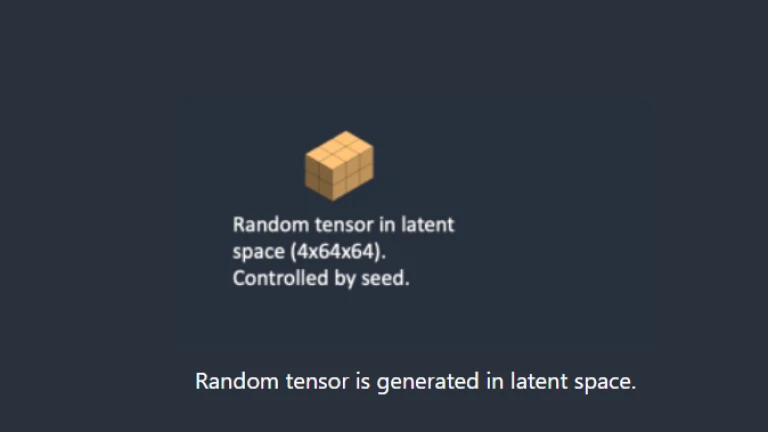
Stable Diffusion AI’s latent space is 4x64x64, 48 times smaller than an image’s pixel space. The latent space is where all of the forward and reverse diffusions we discussed take place.
Consequently, during training, a random tensor in latent space is produced rather than a noisy image (latent noise). Instead than causing noise to distort an image, latent noise distorts the image’s representation in latent space. The reason for doing so is that because the latent space is smaller, it is much faster.
Why is Latent Space Possible?
Why, one might wonder, can the VAE compress an image without losing any of its information into the much smaller latent space? Unsurprisingly, natural images are not random, which is the cause. They occur frequently: A face has a specific spatial arrangement for the mouth, cheek, noise, and eyes. A dog has four legs that are shaped specifically.
In other words, images’ great degree of dimension is artifice. However, without losing any information, natural images can be easily compressed into the much smaller latent space. The manifold hypothesis is what machine learning researchers refer to as.
Reverse Diffusion in Latent Space in Stable Diffusion AI
In Stable Diffusion AI, latent reverse diffusion operates as shown below:
- It generates a latent space matrix at random.
- The latent matrix’s noise is estimated via the noise predictor.
- The latent matrix is then adjusted by the estimated noise.
- Repeat steps 2 and 3 up to a specified sampling step.
- The latent matrix is transformed into the final image via the VAE decoder.
What is VAE File?
Stable Diffusion v1 uses VAE files to enhance the eyes and faces. They are the autoencoder’s decoder, as we previously discussed. The model can paint greater details by further adjusting the decoder.
You may have guessed that what I said earlier is not totally accurate. Since the fine features were not retrieved by the original VAE, information is lost when a picture is compressed into the latent space. The VAE decoder is in charge of painting the finer details.
Conditioning
We’re still not sure where the text prompt fits into the picture, though. Stable Diffusion is not a text-to-image model without it. Without any influence over it, you will either see a cat or a dog.
This is where training comes into play. The goal of conditioning is to direct the noise predictor so that, after removing from the image, the anticipated noise will give us what we desire.
Text Conditioning
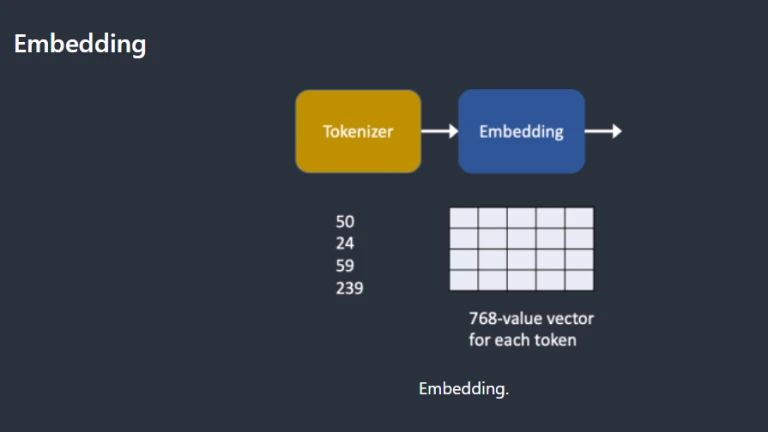
The noise predictor is supplied a text prompt as seen in the overview below. Each word in the question is first transformed into a token number by the tokenizer. The embedding, a vector of 768 values, is then created for each token. (Yes, you used the same same embedding in AUTOMATIC1111) The text transformer then transforms the embeddings so they are prepared for the noise predictor to use.
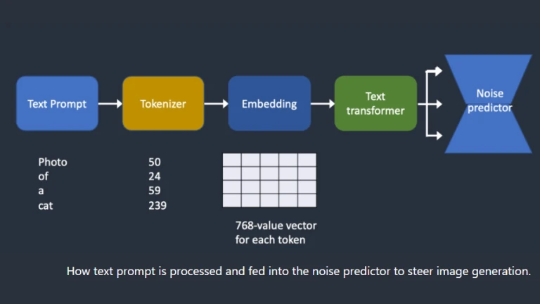 How text prompt is processed
Let’s now examine each component more closely. If you feel that the high-level summary presented above suffices, you can move on to the next section.
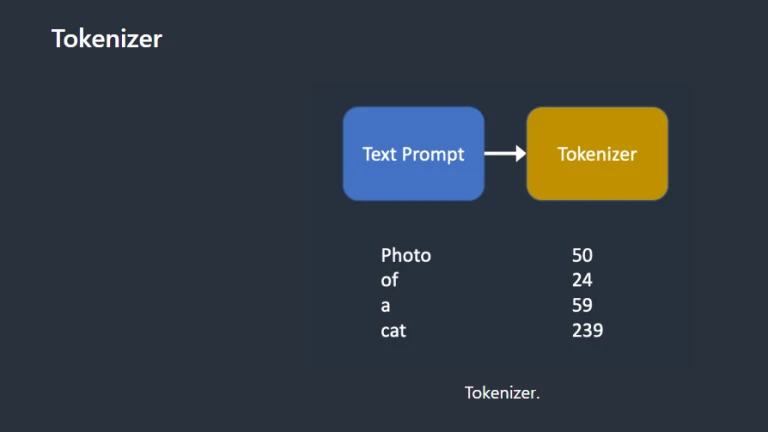 Tokenizer
A CLIP tokenizer first tokenizes the text prompt. Open AI created the deep learning model CLIP to generate text descriptions of any photos. The tokenizer in Stable Diffusion v1 is CLIP.
The way a computer comprehends language is through tokenization. While computers can only read numbers, humans can read words. For this reason, text prompt words are first changed into numbers.
Only words that have been observed during training can be tokenized by a tokenizer. For instance, the CLIP model has “dream” and “beach,” but not “dreambeach.” The words “dreambeach” would be split into the tokens “dream” and “beach” by a tokenizer. Consequently, not all words have the same meaning.
The space character is also a token, which is another small print. In the example above, the words “dream beach” and “[space]beach” are produced twice. These tokens differ from those created by “dreambeach,” which combines the words “dream” and “beach” (without space before beach).
A prompt for the Stable Diffusion model can only include 75 tokens. (You now understand that it differs from 75 words!)
Embedding
ViT-L/14 Clip model from Open AI is utilised in stable diffusion v1. Embedding is a vector with 768 values. Each token has a distinct embedding vector of its own. The CLIP model, which was trained, corrects embedding.
Why is embedding necessary? It’s because we want to take advantage of the fact that some words are closely related to one another. For instance, because “man,” “gentleman,” and “guy” can all be used practically identically, their embeddings are essentially equivalent. All three impressionist painters—Monet, Manet, and Degas—used different techniques. The names’ embeddings are similar but not identical.
 Embedding
This is the embedding that we discussed when a style was activated by a keyword. Embeddings have magical powers. Finding the appropriate embeddings, also known as textual inversion, allows for the triggering of arbitrary objects and styles, according to research.
Feeding Embeddings to Noise Predictors
The text transformer must perform additional processing on the embedding before passing it to the noise predictor. The transformer functions as a global conditioning adaptor. Although the input in this instance is text embedding vectors, it may very well be class labels, pictures, or depth maps. The transformer offers a way to incorporate several conditioning modalities in addition to further processing the input.
The noise predictor utilises the output of the text transformer repeatedly across the U-Net. Through a cross-attention mechanism, the U-Net absorbs it. That is how the words in the prompt came to be combined and connected. In order for Stable Diffusion to know to paint a man with blue eyes and not a blue guy with eyes, the prompt “A man with blue eyes” needs cross-attention between “blue” and “eyes.”
A side note: Hypernetwork hijacks the cross-attention network to introduce styles as a way to fine-tune Stable Diffusion models.
Step by Step: Stable Diffusion
Now that you are familiar with all the inner workings of stable diffusion, let’s go through some examples of what actually occurs.
Text-to-Image
Giving Stable Diffusion a text prompt causes it to return an image in text-to-image.
In the first step, a random tensor is produced in the latent space through stable diffusion. By changing the random number generator’s seed, you can customise this tensor. You will consistently receive the same random tensor if you set the seed to a specific value. Therefore, our representation exists in latent space. But for now, it’s just noise.
 Step 1
In Step 2, the noise predictor U-Net inputs a latent noisy image and a text prompt to forecast noise in latent space (a 4x64x64 tensor).
 Step 2
Subtract the latent noise from the latent picture in step 3. Your new latent image is now this.
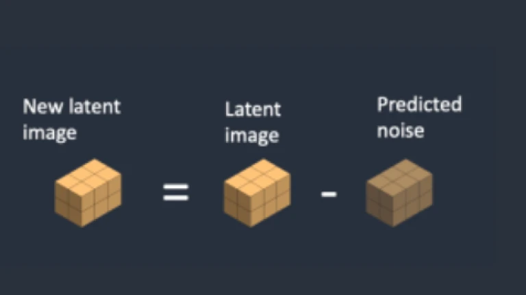 Step 3
For a predetermined number of sample steps, such as 20, steps 2 and 3 are repeated.
Step 4: The latent image is finally converted back to pixel space by the VAE decoder. The result of performing Stable Diffusion is this image.
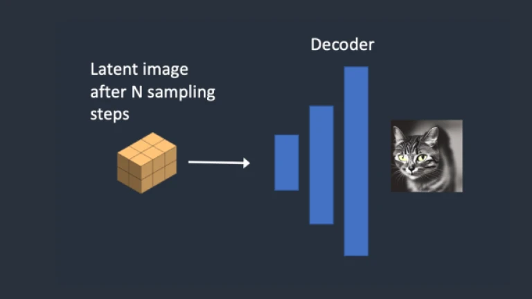 Step 4
Image to Image
A technique first suggested in SDEdit is called image-to-image. We have image-to-image for Stable Diffusion using SDEdit, which can be applied to any diffusion model (a latent diffusion model).
An input image and a text prompt are provided in image-to-image. The input image and text prompt will both influence the resulting image. For instance, image-to-image may transform the following amateur sketch into a professional one using the instruction “picture of perfect green apple with stem, water drops, and dramatic lighting” as inputs:
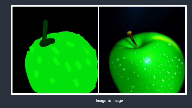 Image to Image
The input image is encoded into latent space in step 1.
Step 2: The latent image is given noise. How much noise is added is controlled by denoising strength. No noise is added if it is 0. If it is 1, the latent picture is completely randomised by adding the maximum amount of noise.
Step 3: The noise predictor U-Net predicts the noise in latent space using the latent noisy image and text prompt as inputs (a 4x64x64 tensor).
Step 4: The latent noise is subtracted from the latent image in step four. Your new latent image is now this.
For a specific number of sample steps, such as 20, steps 3 and 4 are performed 20 times.
Inpainting
In reality, inpainting is just a particular instance of image-to-image. Thus, the areas of the image you wished to paint over have noise added to them. Denoising strength has a comparable effect on noise level.
Depth-to-Image
As an improvement to image-to-image, depth-to-image creates new images with more conditioning by using a depth map.
In Step 1, input image is encoded to latent state.
In Step 2, the depth map is estimated from the input image by MiDaS (an AI depth model).
As part of Step 3, the latent image is given noise. How much noise is added is controlled by denoising strength. No noise is added if the denoising strength is set to 0. The latent picture is turned into a completely random tensor if the denoising strength is set to 1.
Step 4: Using the depth map and the text prompt as conditions, the noise predictor predicts noise in the latent space.
Take the latent noise out of the latent image in step 5. Your new latent image is now this.
The number of sampling steps is determined by repeating steps 4 and 5.
CFG Value
Without defining Classifier-Free Guidance (CFG), a value that AI researchers experiment with daily, this article will fall short of its goal. We must first discuss classifier guidance, which was its predecessor, in order to comprehend what it is.
Classifier Guidance
Diffusion models can also integrate classifier guidance so that a label can be used to direct the diffusion process. For instance, you can direct the reverse diffusion process to produce images of cats by using the class label “cat”.
A parameter for regulating how closely the diffusion process should follow the label is the classifier guiding scale.
The images created by the diffusion model with classifier guidance would be biassed towards extreme/unambiguous examples of that category. For instance, if you ask the model for a cat, it will only provide an image that is clearly of a cat.
The parameter classifier guidance scale determines how powerful this guidance is.
Classifier-Free Guidance for Stable Diffusion AI
Although classifier advice set records, it still requires a second model to serve as guide. Training has been made more challenging by this.
To obtain “classifier guidance without a classifier,” as its creators put it, one must use classifier-free guidance. They suggested utilising image captions to train a conditional diffusion model, just like the one we covered in text-to-image, in place of class labels and a separate model for guiding.
In order to achieve the so-called “classifier-free” (i.e., without a separate image classifier) guidance in picture formation, they also added the classifier component as conditioning of the noise predictor U-Net.
This direction is provided with a text prompt for text-to-image.
CFG Value
How can we regulate the degree to which the guidance should be followed now that we have a classifier-free diffusion process through conditioning?
The classifier-free guidance (CFG) scale is a parameter that regulates how much the text prompt influences the diffusion process. When it is set to 0, the image production is unconditional (i.e., the prompt is disregarded). Thus, the diffusion is directed toward the prompt by a higher value.
Follow us on Instagram: @niftyzone